Author Archives: AR-CHI-VES

Tech #2 : What is the x64?

그냥 지나치고 넘어 갈 수도 있는 CPU 관련 내용을 재 정리 해 봅니다.

우선, x64란?

32bit Architecture(IA-32)를 64bit로 확장시킨 Architecture, 또는 그것과 호환성이 있는 기술의 총칭.

Intel은 자사 Architecture를 “EM64T(Intel Extended Memory 64 Technology”라고 하고, AMD(Advanced Micro Devices, Inc.)는 “AMD64 ISA”라고 하고 있습니다. x64 대응 Processor를 개발하고 있는 건 위의 Intel과 AMD입니다.

x64의 설계는 기존 32bit Architecture의 진화의 연장선상에 있고, x64는 차세대 Computing으로의 벽을 부수고, 과거의 자산을 활용하는 방법을 제공하고 있습니다. 즉, x64는 새로운 64bit Solution을 도입가능하도록 함과 동시에 기존의 32bit Solution에 대한 지금까지의 투자를 보완하기 위한 개념에서 탄생된 새로운 형태의 Technology입니다.

64bit Technology가 필요한 이유

64bit 환경을 필요로 하고 있는 것은 고성능을 필요로하는 대용량 물리 Memory와 가상 Memory를 사용하는 Application. 32bit로 관리 가능한 Addressing Area는 근본적으로 4GB까지 제한되어 버리고, 또, 많은 32bit OS가 Address 가능한 영역도 2GB까지 제한하여 이이상의 Memory영역을 사용하고 싶은 Computing 기능의 강화를 필요로하는 User는 64bit 환경으로 전환해야만 할 필요성이 있죠. 그로 인해 기존 자산인 32bit 환경을 어떻게 해야 할지 하는 문제가 발생합니다.

AMD64와 EM64T의 64bit Technology에 의해 일부 또는 모든 Application의 Software, Hardware를 32bit에서 64bit로 서서히 전환 가능하게 되었습니다.

AMD와 AMD64

AMD는 오래전부터 Intel 호환 Processor 개발을 했던 America의 Maker. 회사의 기술 Level은 상당히 높았고, Original의 x86계 Processor 개발 Maker였던 Intel을 놀라게 할 정도의 존재 가치가 되어 가고 있습니다. 그 대표적인 기술이 AMD64 Platform. AMD64는 IA-32등에서 사용되었던 x86 명령 Set을 확장, 64bit Platform로, Intel의 EMT64에 앞서, 기존 x86 Solution과의 완전호환성을 가지면서, 64bit 성능을 제공하도록 설계되어 있습니다.

2003년 4월, Server 혹은 Workstation 용의 AMD Opteron Processor가 등장. 더불어 AMD는 처음으로 Windows 대응 Desktop/Mobile Processor인 AMD Athlon 64 Processor를 2003년 9월에 발표했습니다. 이 때 Code Name “Hammer”라고 했던 AMD64는 2005년엔 “AMD64 Platform”으로, “x86-64″라는 64bit 확장 기능에 대해서 “AMD64 ISA” (AMD 64 Inform Set Architecture)라고 하게 되었습니다.

Intel과 EM64T

Intel은 업계 최고의 America 최대의 Processor Maker. Intel은 차세대 Processor로서, Hi-end 64bit 전용 Processor인 Itanium/Itanium2를 개발하고 있었지만, Itanium2는 기존 32bit Architecture와는 Hardware Level의 호환성이 없었습니다.

그 때 Rival 기업인 AMD가 “기존 32bit Architecture에 64bit 기능을 추가한다”라는 새로운 전략을 내세웠기 때문에, 그것에 대항하기 위해 EM64T라는 AMD의 AMD64와 동등한 호환성의 높은 시술을 발표했습니다. 물론, Intel도 기존의 32bit Architecture에 64bit 확장기능을 추가하는 것을 전부터 연구하고 있었습니다. 그러나, 준비가 되기도 전에 AMD가 선수를 치는 형식이 되고, 결과적으로 Intel의 EM64T는 AMD보다 한발 늦게 시장에 투입되게 되었습니다.

2004년 2월, Intel은 Dual Processor Server/Workstation 용으로 Intel Xeon Processor 개발 Code Name “Nocona” 또는 “Potomac” (Xeon MP Processor 개발 Code Name), 그리고, Single Processor “Prescott” 위 3개의 IA-32 Processor에 Intel EM64T를 탑재한다고 발표했습니다.

EM64T의 기술은 Pentium4 또는 Xeon Processor (6xx Sequence의 Pentium4 Processor)부터 탑재되기 시작했습니다.

x64 기술의 Merit

기존 x86환경, 또는 64bit 전용의 환경보다 x86환경에서 잘 동작하는 Application 혹은 Case Study는 많이 있습니다. 64bit Native Code로 해도 이점이 없는 Application에 대해서는 변환작업이 필요없고, 그 대로 x64 환경에서도 성능을 Full로 발휘 가능합니다. 특히, Modeling Simulation, 통계, 재무분석, 화상, Video, 신호처리, 물리학, 의학연구, Telecom, 암호화, 압축등 수학적정산과 부동소수점연산기능을 필요로하는 Application에 유리합니다. 게다가,의사결정지원, 검색, 색인, Document, Contents관리, 음성인식등, 대용량 및 고성능의 Database기능을 필요로하는 Application을 비롯, Computer 지원 설계, 제조, Engineering(CAD, CAM, CAE), Digital 음악제작 혹은 Video 편집, Digital Contents 작성, Realtime Media Streaming Solution등의 Application에도 유리하게 적용됩니다.

Tech #1 : What is the 64bit?

Leave a reply

Processor PC의 세계는 4bit 시대로부터 시작하여, Z80에 대표되는 8bit, 8086과 MPU68000에 대표되는 16bit, i386과 Pentium에 대표되는 32bit로 발전되어 왔다. 그리고, 64bit 시대에 접어들어 “64bit화”가 진행되고 있다.

64bit란?

간단하게 말하자면, Bit(1또는 0인 Computer의 최소단위)의 수가 64개가 나열되어 있는 것. 이 64개의 1과 0을 조합하여 표현 가능한 수의 폭은 2⁶⁴이 됩니다. 각 bit수와 값을 Table 1로 정리하면.

Table 1 Bit수와 값의 범위
Bit수	값	값의 범위(Addressing의 범위)	Size
4bit	2⁴	0 ～ 16［0xF］	16byte
8bit	2⁸	-128 ～ +127 0 ～ 255［0xFF］	256byte
16bit	2¹⁶	-32768 ～ +32767 0 ～ 65535［0xFFFF］	64Kbyte
32bit	2³²	-2147483648 ～ 2147483647 0 ～ 4294967295［0xFFFFFFFF］	4Gbyte
64bit	2⁶⁴	-9223372036854775808 ～ 9223372036854775807 0 ～ 18446744073709551615［0xFFFFFFFFFFFFFFFF］	16Ebyte

이 값의 범위를 비교해 보면, 64bit라는 수가 엄청난 크기의 값이라는 걸 금방 알 수 있을 겁니다. 64bit에서 표현가능한 Address 범위는 16Ebyte나 됩니다. 참고로 Ebyte를 참고하기 위해 아래 표를 확인.

Table 2 값의 단위와 Binary 값
단위	값	Binary 값
Kilo(K)	1,000	1,024
Mega(M)	1,000,000	1,048,576
Giga(G)	1,000,000,000	1,073,741,824
Tera(T)	1,000,000,000,000	1,099,511,627,776
Peta(P)	1,000,000,000,000,000	1,125,899,906,842,624
Exa(E)	1,000,000,000,000,000,000	1,152,921,504,606,846,976

물리 Address와 가상 Address의 범위

위에서 64bi의 Address범위는 16EByte라고 설명했지만, 현재의 64bit 대응 Processor으로는 모든 Address범위를 다루지 못 합니다.

Itanium2 Processor로 대표되는 Intel IA-64 Architecture에서는 50bit가 물리 Address 범위입니다. 또, AMD Opteron등의 AMD64 Architecture에서는 40bit까지의 물리 Address와 48bit까지의 가상 Address가 Support되고 있습니다. 이 40bit라는 값은 1TByte까지의 물리 Address범위를 cover하고 있는 것이 됩니다.

또, 이 범위에 관해서는 Processor 혹은 OS 종류에 따라 달라지기 때문에 주의 할 필요가 있습니다. 실제의 64bit 대응 Processor에서 다룰 수 있는 물리 Address 범위는 Table 3에 있습니다.

Table 3 주요 64bit 대응 Processor의 물리 Address 범위
Processor	Architecture	물리Address	가상Address
Intel Itanium2	IA-64	50bit	64bit
Intel Itanium	IA-64	44bit	54bit
AMD Opteron	AMD64	40bit	48bit
AMD Athlon 64	AMD64	40bit	48bit

왜 64bit를 필요로하는가?

Computer 세대가 발전에 나가는 것에 맞춰, bit수도 증가해 왔습니다. 그럼, 왜 이와같이 bit수를 증가시켜야만 했을까요. 그것은 기술의 발달과 함께 처리해야하는 Data량이 증가하여, Computer에 실장되어 있는 Memory의 상한선에 다다르게 되었기 때문입니다.

이미 Memory는 32bit의 한계범위에 있는 4GByte(2³²Byte)에 도달 해 버렸습니다. 일반적인 32bit Computer에서 4GByte 이상의 Memory를 직접(물리적으로) Access 접근할 수 없습니다. 그러나, Hi-End의 x86 Multiple Processor System에서는 이미 이 4GByte의 폭을 넘어서 있습니다.

Intel Server용의 Xeon Processor (Nocona 혹은 일부의 Prescott Core)에서는 “Intel Extended Server Memory Architecture”라고 하는 확장 기능으로 36bit의 물리 Address 공간을 Support하고 있고, 최대 64GByte까지의 Memory 영역을 다룰 수 있습니다. 그러나, 이것은 물리 Address의 한계로의 근본적인 해결책은 아닙니다.

이런 문제를 해결하기 위해서, 64bit로 가기위한 준비의 필요성이 부각되고 있습니다.

64bit는 32bit의 배

64bit는 32bit의 배의 bit폭이므로, 처리속도 및 다룰 수 있는 Data양도 배가 된다고 기대하기 쉽지만, 그렇지 않습니다. 이런 잘못된 인식을 갖지 않도록 64bit에 대해서 정확하게 이해하고 있지않으면 안되지요.

Linux #2 : About Memory on Linux

Leave a reply

System에 장애가 발생 했을 시, 문제를 잘 파악하는게 중요한 Point가 되고,
장애의 원인을 정확하게 파악하고 있다면, 무엇을, 누가, 어떻게 해야 하는지가 명확 해 집니다.
그렇지 못하다면, 인적, 금전적 Resource가 낭비되는 건 당연하구요.

System 상에서 장애 원인을 파악하기 어려운 부분 중의 하나가 Memory인데, 이는 OS 관련 문제 중
20% ~ 30%를 차지하고 있을 정도죠. Memory Trouble은 어려 복잡한 문제가 혼합되어 일어나는데
그 문제는 Application, Middle-Ware, OS, Hardware와 관련되어 더욱더 해결하기 어려워지죠.

일단 Memory를 확인 하기 위한 Command부터 숙지 할 필요가 있을 듯 하네요.
대표적으로 free, vmstat, sar, top, ps가 되죠.

우선,

free : 간단하게 메모리를 파악할 수 있으나, 보기 애매한 부분이 있죠.
vmstat : Memory 상황 및 CPU 사용률도 같이 파악 할 수 있으나, Option이 다양하지 않아 특정
Period에 고부하가 발생 했을 시에는 적합하지 않을 수 있어요.
sar : 위 나열된 Command 중에 가장 취득정보가 많으나,  약간 부적절한 부분도 있어 Memory 감시
관점에서는 vmstat보다 좀 떨어집니다.
top : real time으로 볼수 있는 tool인데, 여러가지 기능이 있고 Log 기록도 가능하죠
( - b batch mode 시)
ps : top과 같이 real time으로 볼 수 있는 tool이고, 여러 Option이 있는데 습관에 따라 쓰는 것
만 쓰게 된다는 예를 들면 "ps ax", "ps aux", "ps -elf" 등이죠.

그럼, 실제 사용 시를 확인 해 볼까요?

# free total used free shared buffers cached Mem: 4046504 3453500 593004 0 111468 1755760 -/+ buffers/cache: 1586272 2460232 Swap: 4192912 1178400 3014512

각 부분의 의미를 간단하게 설명 하자면

[Mem] total : Total Physical Memory size
[Mem] used : Total Physical Memory size - Free memory size
[Mem] free : 현재 사용되고 있지 않은 여유 Memory
[Mem] shared : 항상 0이고, 현재 사용되고 있지 않음.
[Mem] buffers : File등의 Meta data를 Cache하고 있는 Physical Memory size
[Mem] cached : File의 Real Data를 Cache하고 있는 Physical Memory size
[-/+ buffers/cache] used- : buffers, cached를 포함하고 있지 않은 used size
[-/+ buffers/cache] free+ : buffers, cached를 포함한 free size
[Swap] total : Total Swap size
[Swap] used : Total Swap size - Free size
[Swap] free : 사용하고 있지 않은 Swap size

여기서 [Mem] Free는 “남아있는 Memory Size”가 아닌, 어떠한 용도로도 사용되고 있지 않은
Physical Memory Size라고 생각하면 되고, 이는 [Mem] Free가 적다 -> 남아 있는 Memory size가
적다 -> 이용가능한 Memory size가 부족하다와 같은 발생을 막기 위함입니다. 따라서, 단순하게
Physical Memory를 추가해도 언젠가는 [Mem] Free가 이전과 같아 지지요.

결론적으로 System 전체의 Memory 사용량의 감시는 [Mem] Free을 판단 기준으로 하는 것이 아니라, 사용가능한 Physical Memory Size로 계산 할 필요가 있죠.

System의 이용가능한 Memory size의 계산은 Linux의 Page Cache에 대해서 이해 할 필요가 있는데,
Linux는 HDD등의 Storage에 저장되어 있는 Data에 대해서 Read / Write 시에 확보 했던 Memory를
Page Cache라는 형태로 보존 합니다.

CPU는 Storage의 Data를 직접 Read 할 수 없어서 Storage Data는 우선 Memory에 Load를 합니다.
이렇게 Read한 Data를 Page Cache로서 재이용합니다. 일단 Load 해 두면 Page Cache는 Read/Write를 Storage에서 Read 해 올 필요가 없으므로 고속처리가 가능하죠.

Page Cache는 새로 Storage Data를 Read/Write로 인해 Memory를 추가 할 필요가 없는 한, Memory를 release 하지 않으므로, 일반적으로 System이 가동하고 있는 것 만으로도 [Mem] Free는 Page Cache로서 계속 활용되고 어느 정도까지 계속 줄어들게 되죠. 서버마다 다르긴 한데, 어떤 건 150MB까지 또 어떤건 202MB 제 경험상 동일한 Application이 계속 돌고 추가 되지 않는 한 항상 같은 Free Memory size를 유지하게 됩니다. 따라서, [Mem] Free가 50MB가 계속 유지된다고 해서 반드시 걱정 할 필요가 없는 거지요.

이 Page Cache는 사용중이 아닌 Storage와 Data Sync 되어 있으면 바로 Release 할 수 있고, Page Cache에 대한 Write가 있을 경우엔 일시적으로 Unsynchronized 상태가 되지만, Storage와의 Sync는 정기적으로 이루어지고 있어 시간이 지나면 Release 가능한 상태가 됩니다. 즉, Page Cache는 “System이 다른 용도로 재이용 가능한” Memory를 포함하고 있죠.

이용 가능한 Physical Memory Size를 free command를 통해 계산 하는 방법

free command에도 어느정도는 Page Cache를 의식하여 개량되어 있고, 그것이 used – 와 free +입니다.

Buffers와 Cached는 Page Cache이고, 정확하게는 Buffers는 Cached에 SwapCached를 추가한 것이 Page Cache의 Total이지만, free command에서는 SwapCached가 표현되지 않죠. 그림을 보면, Buffers와 Cached를 합친 것을 used에서 뺀(used-), free를 더한 (free+)로 보다 현실적인 Physical Memory size와 이용가능한 Physical Memory size를 출력하고 있죠. 따라서, 이 두 수치를 참고하면 됩니다.

그렇다고 해서, System이 이용가능한 Memory size를 파악하기엔 부족하죠. 앞에서, Page Cache를 다른 용도로 재이용하기에는 “Storage와 Sync하고 있음”이라는 조건이 있었죠. Buffers와 cached에는 당연히 “Storage와 Unsynchronized” Page Cache가 포함되어 있죠. 그래서, free+는 실제 이용가능한 Memory size보다 좀 더 부풀려져 있게 되고, 아래와 같이 표현 가능하죠.

free < 실제 사용가능한 Memory size < free+

Physical Memory Status 확인 방법

그럼, Storage와의 Sync 정보까지 포함한 Memory 사용상태 감시를 위해서는 Active와 Inactive를 감시하면 됩니다.

Active와 Inactive는 vmstat -a 나 cat /proc/meminfo를 통해 취득 가능하죠.

# vmstat -a procs -----------memory---------- ---swap-- -----io---- --system-- -----cpu------ r b   swpd   free inact active   si   so    bi    bo   in   cs us sy id wa st 0 0 1178400 534328 805388 2502796    0    0   161   159    0    0 7 2 89 1 0

$ cat /proc/meminfo
MemTotal:      4046504 kB
MemFree:        424364 kB
Buffers:        117508 kB
Cached:        1845500 kB
SwapCached:     726764 kB
Active:        2610468 kB
Inactive:       803068 kB
HighTotal:           0 kB
HighFree:            0 kB
LowTotal:      4046504 kB
LowFree:        424364 kB
SwapTotal:     4192912 kB
SwapFree:      3014512 kB
Dirty:            9800 kB
Writeback:           0 kB
AnonPages:     1448396 kB
Mapped:          24508 kB
Slab:           152152 kB
PageTables:      27492 kB
NFS_Unstable:        0 kB
Bounce:              0 kB
CommitLimit:   6216164 kB
Committed_AS: 4136824 kB
VmallocTotal: 34359738367 kB
VmallocUsed:    264576 kB
VmallocChunk: 34359473651 kB
HugePages_Total:     0
HugePages_Free:      0
HugePages_Rsvd:      0
Hugepagesize:     2048 kB

Active는 Page Cache나 Anonymous Page 중 최근 이용 했거나 아직 Storage와 Unsynchronized인 Release 할 수 없는 Page이고, Inactive는 Page Cache나 Anonymous Page 중 마지막으로 Access 된 이후 어느 정도 시간이 지나 Storage와의 Sync가 완료되어 바로 Release 할 수 있는 Page이죠. 따라서, /proc/meminfo의 MemFree와 Inactive를 더한 것이 정확한 이용 가능 Memory size가 됩니다.
아참 여기서 Anonymous Page란 주로 User Process가 이용하고 있는 Page로, ps 등으로 취득가능한 RSS로 표시되는 값입니다. 실제, Shared Memory가 Page Cache에 포함되어 있거나 해서, 정확하게 파악하는 것은 상당히 번거로운 일이죠.

실제 이용 가능한 Memory size ≒MemFree + Inactive

Additional information : Kernel Tuning to control the Page Cache

Page Cache가 항상 남아있어 이를 Release 하고 싶은 경우 drop_caches 를 사용하면 되죠. drop caches는 지금 사용되고 있지 않은 Storage와 Unsynchronized Page Cache나 Slab Cache를 MemFree로 Release 합니다.
즉, MemFree ≒ 이용 가능한 Memory가 되죠.

아참 여기서 Slab Cache란 Directory의 Meta Data 정보를 수용하는 dentry나 File의 Meta Data 정보를 수용하는 inode 구조체등을 Cache하고 있는 Kernel내의 Memory 영역입니다. 이는 Page Cache와 별도로 Kernel 안에 확보되어 있고, Storage와 Sync되어 있으면 Release도 언제든지 가능합니다.

아래는 사용방법 입니다.

1. Default 상태로 # echo 0 > /proc/sys/vm/drop_caches 2. Page Cache만 Release # echo 1 > /proc/sys/vm/drop_caches 3. Slab Cache를 Release # echo 2 > /proc/sys/vm/drop_caches 4. Page Cache와 Slab Cache를 Release # echo 3 > /proc/sys/vm/drop_caches

위 drop_caches에 설정 한 parameter는 지속되지 않으므로 필요에 따라 실행해야 합니다.

이 글은 아래 Link의 글을 참조하였습니다.
http://www.atmarkit.co.jp/flinux/rensai/tantei01/bangai01a.html

Network #1 : Load Balancing : DSR (Direct Server Return)

2 Replies

1. What is the DSR(Direct Server Return) Load Balancing?

The type of Load Balancing is typically SLB and DSR, the DSR is when client request, which is balanced through L4 switch, is returning, it doens’t pass through L4 switch again that means returning directly.

Using SLB is as below,

Internet → A → L3 Switch → B  → L4 Switch → C → Web Server → C → L4 Switch →
 B → L3 Switch → A → Internet

The point is the Client Request and Server Response pass through L4 switch.
Using DSR is returning directly from the server as below,

Internet → A → L3 Switch → B → L4 Switch → C → L2 Switch → D → Web Server 1 → D →
 L2 Switch → C → L3 Switch → Internet

2. How to configure the DSR(Direct Server Return) on Linux?

You need to add and configure the Loopback device with L4 for DSR.

/sbin/ifconfig lo:0 xxx.xxx.xxx.xxx netmask 255.255.255.255
# ifconfig eth0 Link encap:Ethernet HWaddr 00:50:56:92:5E:B9 inet addr:10.0.0.151 Bcast:10.0.0.255 Mask:255.255.255.0 inet6 addr: xxxx::xxxx:xxxx:xxxx:xxxx/64 Scope:Link UP BROADCAST RUNNING MULTICAST MTU:1500 Metric:1 RX packets:1216814699 errors:0 dropped:0 overruns:0 frame:0 TX packets:1098502538 errors:0 dropped:0 overruns:0 carrier:0 collisions:0 txqueuelen:1000 RX bytes:286063316490 (266.4 GiB) TX bytes:580239909610 (540.3 GiB) Base address:0x2000 Memory:d8920000-d8940000 lo Link encap:Local Loopback inet addr:127.0.0.1 Mask:255.0.0.0 inet6 addr: ::1/128 Scope:Host UP LOOPBACK RUNNING MTU:16436 Metric:1 RX packets:420991723 errors:0 dropped:0 overruns:0 frame:0 TX packets:420991723 errors:0 dropped:0 overruns:0 carrier:0 collisions:0 txqueuelen:0 RX bytes:720576542847 (671.0 GiB) TX bytes:720576542847 (671.0 GiB)
lo:0 Link encap:Local Loopback inet addr:xxx.xxx.xxx.xxx Mask:255.255.255.255 UP LOOPBACK RUNNING MTU:16436 Metric:1

If you want to add a device for DSR and work permernatly, create the loopback device “ifcfg-lo:0”
if not then you will be creating one.
Excute the following command:

# cd /etc/sysconfig/network-scripts # vi ifcfg-lo:0 DEVICE=lo:0 IPADDR=xxx.xxx.xxx.xxx NETMASK=255.255.255.255 ONBOOT=yes NAME=loopback

Additionally it is necessary to disable invalid ARP replies(misbehaving)

“Linux ARP flux” problem. Linux answers ARP requests on wrong and unassociated interfaces per default. This leads to the following two problems:

ARP requests for the loopback alias address are answered on the HW interfaces (even if NOARP on lo0:1 is set).
If the machine is connected twice to the same switch (e.g. with eth0 and eth1) eth2 may answer ARP requests for the address on eth1 and vice versa in a race condition manner (confusing almost everthing).

This can be prevented by specific arp kernel settings. Take a look here for additional information about the nature of the problem (and other solutions): http://linux-ip.net/html/ether-arp.html#ether-arp-flux.

To fix that generally (and reboot safe) we recommend to include the following lines into /etc/sysctl.conf (2.6 kernel only):

net.ipv4.conf.all.arp_ignore=1 net.ipv4.conf.all.arp_announce=2

The following commands may be used to change the settings interactively during runtime:

# echo 1 > /proc/sys/net/ipv4/conf/all/arp_ignore # echo 2 > /proc/sys/net/ipv4/conf/all/arp_announce

Unfortunately there seems to be no general and simple solution for for kernel 2.4. We recommend currently upgrading to 2.6 kernel in that case, this is probably the easiest way.

Linux #1 : Performance tuning of OpenLDAP #1

1 Reply

1. Tune buffer cache size of Berkely DB

The buffer cache becomes a typical tuning point of MySQL (InnoDB storage engine) and PostgreSQL open source database or even any other commercial databases. Only if some database is working with data, it should avoid the disk I/O and deployment data in memory for faster to get some data is persisted on the files and index. This setting is preferred.

Even in the Berkeley DB library as incoperated into the program, it can maintain the data in the buffer cache frequently like database to act as an independent process. It can configure the buffer cache size on DB_CONFIG file with Berkeley DB files. When the openLDAP starts, the directory information such as entries, indexes is cached.

There are two ways to tune for the buffer cache size.

a) The buffer cache size necessary to load the database via slapadd in optimal time
b) The buffer cache size necessary to have a high performing running slapd once the data is loaded

For (a), the optimal cachesize is the size of the entire database, If you already have the database loaded, this is simply

# cd /usr/local/var/openldap-data # du -ch *.bdb 68K cn.bdb 64K dn2id.bdb 12K entryCSN.bdb 20K entryUUID.bdb 12K gidNumber.bdb 308K id2entry.bdb 8.0K loginShell.bdb 28K memberUid.bdb 28K objectClass.bdb 8.0K ou.bdb 8.0K sn.bdb 40K uid.bdb 8.0K uidNumber.bdb 8.0K uniqueMember.bdb 620K total

in the directory containing the OpenLDAP (default path : /usr/local/var/openldap-data) data.

For (b), the optimal buffer cache is just the size of the id2entry.bdb file, plus about 10% for growth.

For example,

# cd /usr/local/openldap/var/openldap-data # vi DB_CONFIG ... [Example] set_cachesize 0 268435456 1 It will be provided 0.25 GBytes buffer logically and composed one cached area physically [Format] set_cachesize gbytes bytes ncache gbytes : cache size by Gbytes bytes : cache size by Bytes ncache : a mount of cached files

Re-mapping buffer size by new configuration

# cd /usr/local/openldap/var # /etc/init.d/slapd stop # rm -rf __db.* # /etc/init.d/slapd start # lsof __db.003 COMMAND PID USER FD TYPE DEVICE SIZE NODE NAME slapd 1405 ldap mem REG 253,3 335552512 24445661 __db.003

2. Tune log buffer size of Berkeley DB

The log buffer is area that is used to comfirm update or caused by its log buffer space becomes full before writing occurs to the transaction log file, if update request to the Berkeley DB.

For example,

# cd /usr/local/openldap/var/openldap-data # vi DB_CONFIG ... [Example] set_lg_bsize 2097152 By default, or if the value is set to 0, a size of 32K is used [Format] set_lg_bsize lg_bsize lg_bsize : Set the size of the in-memory log buffer, in bytes. ... [Example] set_lg_regionmax 262144 By default, or if the value is set to 0, the base region size is 60KB The log region is used to store filenames, and so may need to be increased in size if a large number of files will be opened and registered with the specified Berkeley DB environment's log manager. [Format] set_lg_regionmax size size : Set the size of the underlying logging subsystem region, in bytes

Re-mapping log buffer size by new configuration

# cd /usr/local/openldap/var # /etc/init.d/slapd stop # rm -rf __db.* # /etc/init.d/slapd start # lsof __db.004 COMMAND PID USER FD TYPE DEVICE SIZE NODE NAME slapd 1405 ldap mem REG 253,3 2359296 24445662 __db.004

Additional information : Log file limits of Berkeley DB by Reference Guide

Log filenames and sizes impose a limit on how long databases may be used in a Berkeley DB database environment. It is quite unlikely that an application will reach this limit; however, if the limit is reached, the Berkeley DB environment’s databases must be dumped and reloaded.

The log filename consists of log. followed by 10 digits, with a maximum of 2,000,000,000 log files. Consider an application performing 6000 transactions per second for 24 hours a day, logged into 10MB log files, in which each transaction is logging approximately 500 bytes of data. The following calculation:

(10 * 2^20 * 2000000000) / (6000 * 500 * 365 * 60 * 60 * 24) = ~221

indicates that the system will run out of log filenames in roughly 221 years.

There is no way to reset the log filename space in Berkeley DB. If your application is reaching the end of its log filename space, you must do the following:

Archive your databases as if to prepare for catastrophic failure
(see db_archive for more information).
Dump and reload all your databases (see db_dump and db_load for more information).
Remove all of the log files from the database environment. Note: This is the only situation in which all the log files are removed from an environment; in all other cases, at least a single log file is retained.
Restart your application.

DB #6 : [MySQL]High Availability and Scalability

Leave a reply

When using MySQL you may need to ensure the availability or scalability of your MySQL installation. Availability refers to the ability to cope with, and if necessary recover from, failures on the host, including failures of MySQL, the operating system, or the hardware. Scalability refers to the ability to spread the load of your application queries across multiple MySQL servers. As your application and usage increases, you may need to spread the queries for the application across multiple servers to improve response times.

cope with + noun : 극복하다. 잘 처리하다
refer to + noun : 관련되다
spread : 분담하다, 분배하다.

There are a number of solutions available for solving issues of availability and scalability. The two primary solutions supported by MySQL are MySQL Replication and MySQL Cluster. Further options are available using third-party solutions such as DRBD (Distributed Replicated Block Device) and Heartbeat, and more complex scenarios can be solved through a combination of these technologies. These tools work in different ways:

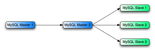
MySQL Replication enables statements and data from one MySQL server instance to be replicated to another MySQL server instance. Without using more complex setups, data can only be replicated from a single master server to any number of slaves. The replication is asynchronous, so the synchronization does not take place in real time, and there is no guarantee that data from the master will have been replicated to the slaves.

Advantages :

MySQL Replication is available on all platforms supported by MySQL, and since it isn’t operating system-specific it can operate across different platforms.
Replication is asynchronous and can be stopped and restarted at any time, making it suitable for replicating over slower links, partial links and even across geographical boundaries.
Data can be replicated from one master to any number of slaves, making replication suitable in environments with heavy reads, but light writes (for example, many web applications), by spreading the load across multiple slaves.

suitable : 적당한, 적절한
partial : 편파적인, 일부분의
boundary : 한계, 경계
sperad : 분배하다. 나누다

Disavantages :

Data can only be written to the master. In advanced configurations, though, you can set up a multiple-master configuration where the data is replicated around a ring configuration.
There is no guarantee that data on master and slaves will be consistent at a given point in time. Because replication is asynchronous there may be a small delay between data being written to the master and it being available on the slaves. This can cause problems in applications where a write to the master must be available for a read on the slaves (for example a web application).

consitent : 일관된, 모순이 없는

Recommended uses :

Scale-out solutions that require a large number of reads but fewer writes (for example, web serving).
Logging/data analysis of live data. By replicating live data to a slave you can perform queries on the slave without affecting the operation of the master.

Online backup (availability), where you need an active copy of the data available. You need to combine this with other tools, such as custom scripts or Heartbeat. However, because of the asynchronous architecture, the data may be incomplete.

live data : using data 사용중인
affect : ~에 영향을 미치다.

Offline backup. You can use replication to keep a copy of the data. By replicating the data to a slave, you take the slave down and get a reliable snapshot of the data (without MySQL running), then restart MySQL and replication to catch up. The master (and any other slaves) can be kept running during this period.

For information on setting up and confliguring replication, see Chapter 15, Replication.

MySQL Cluster is synchronous solution that enables multiple MySQL instances to share database information. Unlike replication, data in a cluster can be read from or written to any node within the cluster, and information will be distributed to the other nodes.

Advantages :

Offers multiple read and write nodes for data storage.
Provides automatic failover between nodes. Only transaction information for the active node being used is lost in the event of a failure.
Data on nodes is instantaneously distributed to the other data nodes.

instantaneously : 즉시

Disadvantages :

Available on a limited range of platforms.
Nodes whithin a cluster should be connected via a LAN; geographically separate nodes are not supported .However, you can replicate from one cluster to another using MySQL Replication, although the replication in this case is still asynchronous.

Recommended uses :

Applications that need very high availability, such as telecoms and banking.
Applications that require an equal or higher number of writes compared to reads.

For information on MySQL Cluster, see Chapter 16, MySQL Cluster.

DRBD(Distributed Replicated Block Device) is a solution from Linbit supported only on Linux. DRBD creates a virtual block device(which is associated with an underlying physical block device)that can be replicated from the primary server to a secondary server. You create a filesystem on the virtual block device, and this information is then replicated, at the block level, to the secondary server.

underlying : 기본적인, 근원적인, 기초를 이루는

Because the block device, not the data you are storing on it, is being replicated the validity of the information is more reliable than with data-only replication solutions. DRBD can also ensure data integrity by only returning from a write operation on the primary server when the data has been written to the underlying physical block device on both the primary and secondary servers.

validity : 타당성, 유효성
reliable : 신뢰하다, 신용하다
ensure : 확실하게 하다. 보장하다
integrity : 고결, 완전한 (상태)

Advantages :

Provides high availability and data integrity across two servers in the event of hardware or system failure.
Ensures data integrity by enforcing write consistency on the primary and secondary nodes.

consistency : 일관성

Disadvantages :

Only provides a method for duplication data across the nodes,. Secondary nodes cannot use the DRBD device while data is being replicated, and so the MySQL on the secondary node cannot be simultaneously active.
Cannot provide scalability, since secondary nodes don’t have access to the secondary data.

simultaneously : 동시에

Recommended uses :

High availability situations where concurrent access to the data is not required, but instant access to the active data in the event of a system or hardware failure is required.

For information on configuring DRBD and configuring MySQL for use with a DRBD device, see Section 14.1. “Using MySQL with DRBD for High Availability”

Heartbeat is a software solution for Linux. It is not a data replication or synchronization solution, but a solution for monitoring servers and switching active MySQL servers automatically in the event of failure. Heartbeat needs to be combined with MySQL Replication or DRBD to provide automatic failover.

The information and suitability of the various technologies and different scenarios is summarized in the table below.

suitability : 적당한
various : 다양한, 여러가지, 색색

MySQL을 사용한다면, MySQL 설치에 가용성 또는 확장성을 고려할 필요가 있습니다. 가용성은 MySQL, OS, H/W down을 포함한 host server의 down으로 부터의 복구하거나, 잘 처리하는 능력과 관련됩니다.
확 장성은 다수의 MySQL servers로 application queries의 load를 분담하는 능력과 관련됩니다. Application이나 사용량이 증가하면, response times의 개선을 위해 다수의 servers로 application queries를 분담할 필요가 있습니다.

아래는 가용성과 확장성의 issues를 해결 가능하는 solutions입니다. 두 개의 solutions은 MySQL의 Replication과 Cluster로 제공됩니다. Further : 더 나아가서, 그 이상의 options은 third-party solutions을 통한 DRBD (Distributed Replicatted Block Device)와 Hearbeat, 그 기술들을 혼합시켜 만든 더 복잡한 시나리오로 처리 가능합니다. 이들 기능은 각기 다른 방법으로 일을 합니다.

MySQL Replication 가능한 상황들과 하나의 MySQL server instance로부터의 data는 다른 MySQL server instance로 Replicate 될 수 있다. 복잡한 설정 없이, 단지 data는 단일 master server에서 다른 많은 slaves로 replicate 할 수 있다. Replication은 비동기로, 그래서 실시간으로 동기화 하지 않고, 제약없이 master로 부터 slaves로 data를 replicate 할 것이다.
Advantages :

MySQL Replication은 MySQL이 지원되는 모든 platforms에서 사용가능하고, 시스템 특성에 따라 작동하고 있지 않은 관계로, 다른 platforms 사이에서도 동작 가능하다.
Replication은 비동기로 언제라도 stop 및 restart 가능하고, 느린 링크들, 편파적인 링크들, 위치적인 한계를 뛰어 넘어 replicating을 하기 적절하게 하고 있다.
Data 는 하나의 master로부터 많은 수의 slaves로 replicate 할 수 있고, 다중의 slaves사이의 부하를 분배하기 위해 많은 reads, 적은 writes (예를 들면, 많은 web applications)의 환경에 적절하다.

Disavantages :

Data는 단지 master에만 쓸 수 있다. 보다 발전된 환경에선 data는 링의 형태의 replcate되고 다중의 master 환경을 설정 할 수 있다.
제 약없이 master와 slaves에게 주어진 시간에 일관되게 data를 보낼 것이다. Replication은 data가 master에 쓰여지게 될 때, slaves에 그것이 가능하도록 작은 지연이 발생하는 비동기 방식이기 때문이다.이것은 master에 쓰고, slaves에서 읽어야만 하는 예를 들면 web application같은 app에서 문제를 야기 시킬 수 있다.

Recommended uses :

Scale-out solutions으로 많은 수의 reads 이나 적은 writes인 예를 들면 web serving.
사용중인 data의 Logging/data analysis. 사용중인 data를 slave로의 replicate 하는 것에 의해 master의 동작환경에 영향을 끼치는 것 없이 queries을 개선 가능하다.
Online backup (가용성), 살아 있는 가용 data의 copy가 필요할 때. 이것들을 준비된 스크립트 또는 Heartbeat 와 같은 다른 tools과 함께 조합 할 필요가 있다.

Offline backup. data를 복사하면서 replication을 사용 할 수 있다. slave로 data를 replcation 하는 것으로 slave를 정지시키거나, Mysql를 가동하지 않고도 data의 snapshot을 얻을 수 있고, MySQL을 재기동 하면, replication이 활성화 된다. Master(또, 어떤 다른 slaves)는 이 기간 동안 계속 가동 가능하다.
replication의 set up 및 설정에 대한 정보는 Chapter 15, Replication을 참조하세요.

MySQL Cluster은 database information 공유로 다중의 Multiple MySQL instances 가능한 동기 solution이다. replication과 다르게, cluster에서 data는 cluster에 포함된 어떤 node에서도 read/write가 가능하고, Information은 다른 nodes로 분산 되게 됩니다.
Advantages :

data storage를 통해 multiple read/write nodes 제공합니다.
Nodes 사이의 자동 failover를 제공. 단 활성 node가 사용하고 있는 transaction information은 failure event로서 손실 됩니다.
Nodes 상의 data는 즉시 다른 data nodes로 분할 됩니다.

Disadvantages :

사용가능한 platforms이 제한 되어 있습니다.
cluster에 포함된 Nodes는 via a LAN으로 접속 해야 합니다; 물리적으로 분리된 nodes는 지원하지 않습니다. 그리고, 하나의 cluster에서 다른 MySQL Replication으로 replcation 가능합니다, 하지만 이 경우의 replcation은 비동기가 됩니다.

Recommended uses :

통신이나 은행과 같은 매우 높은 가용성을 필요로하는 Applications.
reads와 writes가 동일하거나 writes가 많은 비중을 차지하는 Applications.
MySQL Cluster의 정보는 Chapter 16, MySQL Cluster를 참조하세요.
DRBD는 Linux 상의 단지 Linbit(?)으로부터 지원되는 solution이다. DRBD는 primary server로부터 secondary server로 replicate 가능한 virtual block device(기본적인 physical block device로 연관되어진)를 생성한다.
Virtual block device 상에서 filesystem를 만들고, 이 information은 secondary server로 block level로 replicate 된다.

보 관하고 있는 data가 아닌, 그 정보의 유효성을 replicate하고 있는 block device이기 때문에, data만 replication하는 solutions보다 더 신뢰가능하다. DRBD는 또한 primary와 secondary servers 양쪽의 본래의 physical block device로 쓰여질 때, primary server의 write operation으로 부터 return되므로 data의 완전성(고결성)을 보장한다.

Advantages :

두 servers 사이의 hardware의 event 혹은 system failure에서 높은 가용성과 data의 고결성을 제공한다.

Disadvantages :

단 지 nodes 사이에서 data를 복제하기 위한 방법을 제공한다. Secondary nodes는 data를 replicate하고 있는 동안에는 DRBD device를 사용할 수 없고, secondary node상의 MySQL은 동시에 활성화 될 수 없다.

Recommended uses :

data로의 concurrent access 고 가용성 상황에는 적합하지 않지만, system의 evnet 혹은 hardware failure에서 활성 data로의 즉각적인 aceess에는 적합하다.

DRBD 설정과 DRDB device를 사용하기 위한 MySQL 설정 정보는 Section 14.1 “Using MySQL with DRBD for High Availability”를 참조하세요.

Heartbeat 는 Linux를 위한 software solution 입니다. data replication 또는 synchronization solution이 아니라, failure event를 자동으로 active 상태의 MySQL servers를 switching하고 servers를 monitoring하는 solution입니다. Heartbeat는 MySQL Replication 혹은 자동 failover를 제공하는 DRBD와 조합이 필요합니다.

DB #5 : [MySQL][Replication] Improving Replication Performance

1 Reply

As the number of slaves connecting to a master increases, the load, although minimal, also increases, as each slave uses up a client connection to the master. Also, as each slave must receive a full copy of the master binary log, the network load on the master may also increase
and start to create a bottleneck.

If you are using a large number of slaves connected to one master, and that master is also busy processing requests (for example, as part of a scaleout solution), then you may want to improve the performance of the replication process.

One way to improve the performance of the replication process is to create a deeper replication structure that enables the master to replicate to only one slave, and for the remaining slaves to connect to this primary slave for their individual replication requirements. A sample of this
structure is shown in Figure 14.3, “Using an additional replication host to improve performance”.

For this to work, you must configure the MySQL instances as follows:

Master 1 is the primary master where all changes and updates are written to the database. Binary logging should be enabled on this machine.
Master 2 is the slave to the Master 1 that provides the replication functionality to the remainder of the slaves in the replication structure. Master 2 is the only machine allowed to connect to Master 1. Master 2 also has binary logging enabled, and the –log-slave-updates option so that replication instructions from Master 1 are also written to Master 2’s binary log so that they can then be replicated to the true slaves.
Slave 1, Slave 2, and Slave 3 act as slaves to Master 2, and replicate the information from Master 2, which is really the data logged on Master 1.

The above solution reduces the client load and the network interface load on the primary master, which should improve the overall performance of the primary master when used as a direct database solution.

If your slaves are having trouble keeping up with the replication process on the master then there are a number of options available:

If possible, you should put the relay logs and the data files on different physical drives. To do this, use the –relay-log option to specify the location of the relay log.
If the slaves are significantly slower than the master, then you may want to divide up the responsibility for replicating different databases to different slaves. See Section 14.2.4, “Replicating Different Databases to Different Slaves”.
If your master makes use of transactions and you are not concerned about transaction support on your slaves, then use MyISAM or another non-transactional engine. See Section 14.2.2, “Using Replication with Different Master and Slave Storage Engines”.
If your slaves are not acting as masters, and you have a potential solution in place to ensure that you can bring up a master in the event of failure, then you can switch off –log-slave-updates. This prevents ‘dumb’ slaves from also logging events they have executed into their own binary log.

Master에 접속하고 있는 slaves 수가 증가하면, 약간의 부하도 어느정도 증가하여, 각각의 slave가 master로의 client connection을 전부 써 버립니다. 게다가, 각각의 slave는 master의 binary log의 완전한 copy를 받을 필요가 있기 때문에, master network load도 같이 증가하여, bottleneck이 발생 system 전체 성능이 저하합니다.

Scale-out solution등으로 master에 접속하고 있는 slave 수가 많을 때는, 그것에 맞춰 master의 처리량을 증대 시키기 때문에, Replication process의 performance를 개선할 것을 추천합니다.

Replication process의 performance를 개선하는 방법의 하나로, 보다 깊은 Replication structure를 구성하는 것이 있습니다. 이것은 master가 1개의 slave만 복제를 행하고, 다른 slave는 개별 replication 요구로 대응하는 primary slave에 접속하는 방법입니다. 이 structure sample는 그림, 5.8 “추가 Replication host로 performance 개선”을 참조 해 주세요.

이것을 실현하기 위해, MySQL instances를 다음과 같이 설정합니다.

Master 1은 primary master로 이 database에 모든 change와 update가 write됩니다. Binary logging은 이 machine에서 실행가능합니다.
Master 2는 Master1의 slave입니다. Master 1은 replication structure에 있어, Replication의 기능성을 slave의 잔여분으로 제공합니다. 여기서 Master 2는 Master 1에 단일 접속하는 machine입니다. Master 2는 binary logging가 가능한 상태입니다. –log-slave-updates option으로 Master 1으로부터 복제지시가 Master 2의 binary log에 write되고, 이것에 의해, 양자가 slave 복제하게 됩니다.
Slave 1, Slave 2, Slave 3는 Master 2의 slave로써 가동되고, Master 2로부터 정보를 복제하지만, 실제는 Master 1의 log data입니다.

이 solution은 primary master의 client load뿐만이 아니라, Network interface load를 줄이는게 가능하고, primary master의 performance 전체를 개선하는 direct database solution으로 활용가능합니다.

Master의 replication process에 있어 문제를 일으키는 slave가 있는 경우에는 다음 option으로 대응합니다.

Relay log와 data files을 가능한 한 물리적으로 독립된 drive에 분리합니다. 그렇게 하기위해, –relay-log option을 사용하여, relay log의 보관장소를 지정합니다.
Slave가 master보다 매우 느린 경우는, database 종류에 맞춰 복제 역활을 다른 slave에 나눠주는 것을 추천합니다. 자세한 내용은 5.3.4. “다른 database로부터 다른 slave로의 replication”을 참조 하세요.
Master transaction을 활용하고, slave가 그 transaction support를 하고 있는 지 어떤지를 확인하기 위해, MyISAM 또는 그 외의 non-transaction engine을 사용합니다. 자세한 내용은 5.3.2 “Storage engine가 다른 master와 slave의 replication”을 참조 하세요

Slaves가 masters처럼 가동하고 있지 않는 상황에서, 대처가능한 방법이 있고, 장애 event 중의 master를 조작 할 수 있는 경우에는, –log-slave-updates option을 사용합니다. 이것은 “dumb(처리능력없음)” slave가 또, 각각의 binary log에 실행했던 event를 기록하는 것을 방지합니다.

DB #4 : [MySQL][InnoDB] Adding and Removing InnoDB Data and Log Files

Leave a reply

This section describes what you can do when your InnoDB tablespace runs out of room or when you want to change the size of the log files.

The easiest way to increase the size of the InnoDB tablespace is to configure it from the beginning to be auto-extending. Specify the autoextend attribute for the last data file in the tablespace definition. Then InnoDB increases the size of that file automatically in 8MB increments when it runs out of space. The increment size can be changed by setting the value of the innodb_autoextend_increment system variable, which is measured in MB.

lternatively, you can increase the size of your tablespace by adding another data file. To do this, you have to shut down the MySQL server, change the tablespace configuration to add a new data file to the end of innodb_data_file_path, and start the server again.

If your last data file was defined with the keyword autoextend, the procedure for reconfiguring the tablespace must take into account the size to which the last data file has grown. Obtain the size of the data file, round it down to the closest multiple of 1024 × 1024 bytes (= 1MB), and specify the rounded size explicitly in innodb_data_file_path. Then you can add another data file. Remember that only the last data file in the innodb_data_file_path can be specified as auto-extending.

As an example, assume that the tablespace has just one auto-extending data file ibdata1:

innodb_data_home_dir = innodb_data_file_path = /ibdata/ibdata1:10M:autoextend

Suppose that this data file, over time, has grown to 988MB. Here is the configuration line after modifying the original data file to not be auto-extending and adding another auto-extending data file:

innodb_data_home_dir = innodb_data_file_path = /ibdata/ibdata1:988M;/disk2/ibdata2:50M:autoextend

When you add a new file to the tablespace configuration, make sure that it does not exist. InnoDB will create and initialize the file when you restart the server.

Currently, you cannot remove a data file from the tablespace. To decrease the size of your tablespace, use this procedure:

1. Use mysqldump to dump all your InnoDB tables.

2. Stop the server.

3. Remove all the existing tablespace files, including the ibdata and ib_log files. 
If you want to keep a backup copy of the information, then copy all the ib* files 
to another location before the removing the files in your MySQL installation.

4. Remove any .frm files for InnoDB tables.

5. Configure a new tablespace.

6. Restart the server.

7. Import the dump files.

If you want to change the number or the size of your InnoDB log files, use the following instructions. The procedure to use depends on the value of innodb_fast_shutdown:

If innodb_fast_shutdown is not set to 2: You must stop the MySQL server and make sure that it shuts down without errors (to ensure that there is no information for outstanding transactions in the logs). Then copy the old log files into a safe place just in case something went wrong in the shutdown and you need them to recover the tablespace. Delete the old log files from the log file directory, edit my.cnf to change the log file configuration, and start the MySQL server again. mysqld sees that no log files exist at startup and tells you that it is creating new ones.

If innodb_fast_shutdown is set to 2: You should shut down the server, set innodb_fast_shutdown to 1, and restart the server. The server should be allowed to recover. Then you should shut down the server again and follow the procedure described in the preceding item to change InnoDB log file size. Set innodb_fast_shutdown back to 2 and restart the server.

이 Session은 InnoDB Tablespace가 Space를 전부 사용해 버리거나, Log files size를 변경하고 싶을 때에 무엇이 가능한 지를 설명하고 있습니다.

DB Tablespace Size를 증설하는 가장 간단한 방법은, 처음부터 이것을 autoextend increment Mode롤 설정하는 것입니다. Tablespace 정의내의 마지막 data file의 autoextend 속성을 지정 해 주세요.
그럼, InnoDB는 영역을 전부 사용해 버렸을때, 그 file size를 자동적으로 8MB Increment 증설. Increment size는, MB 단위로 innodb_autoextend_increment system 변수갓을 설정하는 것으로 변경 가능합니다.

또는, 다른 data file을 추가하는 것으로 tablespsace size를 증가시는 것이 가능합니다. 이 작업을 하기 위해, MySQL Server를 Shutdown 후, innodb_data_file_path의 마지막에 새로운 data file을 추가하는 것으로 tablespace 설정을 변경하고, MySQL Server를 재기동합니다.

만약 최후의 data file이 keyword autoextend로 정의 되어 있다면, tablespace 재설정 순서는 마지막의 data file이 어느 정도의 size까지 증설할지 고려할 필요가 있습니다. table file size를 위해, 그것을 1024 x 1024bytes (=1MB)의 배수 근접치까지 맞추고, 맞춘 size를 innodb_data_file_path내에 명시적으로 지정하세요. 그럼, 다른 data file을 추가하는 것이 가능합니다. innodb_data_file_path 내의 마지막 data file만이 autoextend increment로써 지정 가능하다는 것 기억하세요.

한가지 예를 들면, tablespace가 1개만 autoextend increment data file ibdata1을 가지고 있다고 가정:

이 data file이 오랜시간에 걸쳐 988MB까지 확장되었다고 가정 해 주세요. 여기서, 원래 data file을 Un-autoextend increment로 변경하고, 다른 autoextend increment file을 추가한 후 설정 Line이 있습니다 :

data space설정에서 새로운 file을 추가할 때에는, 그것이 존재하고 있지 않은 지 확인 하세요. InnoDB는 Server를 재기동 할 때 file을 작성, 초기화 합니다.

현재, data file을 tablespace로부터 삭제하는 것은 불가능. tablespace size를 작게하기 위해서는, 아래 방법을 이용하세요:

1. 모든 InnoDB table을 dump하기 위해 mysqldump를 이용하세요.

2. MySQL Server를 정지 해 주세요.

3. ibdata, ib_log files을 포함하는 모든 존재하는 tablespace files을 삭제해 주세요.

만약 그 정보를 backup 하기를원한다면, 당신의 MySQL 설치관련 files을 삭제하기 전에 다른 위치에

모든 ib* files을 copy 하세요.

4. 모든 *.frm 확장자를 가진 files을 삭제 해 주세요.

5. 새로운 tablespace를 설정 해 주세요.

6. MySQL Server를 재기동 해 주세요.

7. dump files을 inport 해 주세요.

InnoDB log files 수와 size를 변경 하고 싶으면, 다음 지시를 따라주세요. 이용 방법은 innodb_fast_shutdown 값에 의해 결정됩니다:

만약 innodb_fast_shutdown이 2로 설정되어 있지 않으면: MySQL Server을 정지하고, Error 없이 shutdown 되었는지 확인 할 필요가 있습니다.(log 안에 미처리 transaction 정보가 없는것을 보증하기 위해) shutdown 시에 문제가 발생했을 경우, tablespace를 복구하기 위해 필요함으로,
오래된 log files을 안전한 장소에 copy 해 두세요. 오래된 log files을 log file directory로부터 삭제하고, log file설정을 변경하기 위해 my.cnf를 편집하고, MySQL server를 재기동 해주세요. mysqld는 log files이 존재하지 않는 것을 확인하고, 새로운 것을 작성하고 있다고 보고 합니다.

만약 innodb_fast_shutdown이 2로 설정되어 있으면: MySQL Server를 shutdown하고, innodb_fast_shutdown을 1로 설정하고, MySQL Server를 재기동 하세요.

MySQL Server는 복구를 허가합니다. 그리고, MySQL Server를 다시 한번 shutdown하고, InnoDB log file size를 변경하기위해 앞에서 설명하고 있는 방법을 반드시 따라주세요. innodb_fast_shutdown을 2로 다시 설정하고, MySQL Server 를 재설정 하세요.

DB #1 : [MySQL][InnoDB] Raw Device 대응에 대해서

Leave a reply

[아래내용은 http://d.hatena.ne.jp/mir/20060825/p1 사이트에서 인용 하였습니다]

Buffer로서도 File로서도, 영역확보 시에 반드시 Access 단위(Page Size 혹은 Sector Size) 1개분 여분을 취득해서, align합니다.
Oracle은 Parameter 혹은 무언가로 설정해서 사용한다는 이야기가 있습니다만(추후 확인), InnoDB의 경우는 이러한 User측의 제어 방법은 없고, Raw Device를 사용여부에 관계없이, Raw Device를 사용하고 있어서 문제없는Code가 실행 됩니다.

Raw Device를 다시 집어보면 Kernel의 IO Buffer를 우회하여 Device에 대해 직접적인 Read/Write를 행하기 위해, Kernel이 Application에게 제공하는 Service 구조라고 할까요.

http://www.linux.or.jp/JF/JFdocs/SCSI-2.4-HOWTO/rawdev.html
http://www.linux.or.jp/JM/html/util-linux/man8/raw.8.html

스스로 Buffering을 하는 Software의 경우, 이 경우가 Overhead가 줄고, “ACID를 위한 동기 Write가 필요”한 경우에 더욱 편리하다고 하네요. (fsync ?)

http://www.atmarkit.co.jp/flinux/rensai/watch2005/watch06b.html

Raw Device가 장래 Linux에서 사라질지 모른다라는 “System Call Open시에 O_DIRECT를 지정하기 위해 Source Code를 바꿔 써야할 필요가….”
만약 그렇게 되면 InnoDB도 Source를 수정하지 않으면 안된다는.. O_RDWR지정 뿐이므로 (O_RDWR ? )

http://dev.mysql.com/doc/refman/5.0/en/innodb-raw-devices.html

You can use raw disk partitions as data files in the shared tablespace. By using a raw disk, you can perform non-buffered I/O on Windows and on some Unix systems without filesystem overhead, which may improve performance.

http://dev.mysql.com/doc/refman/5.0/en/innodb-tuning.html

When using the InnoDB storage engine with a large innodb_buffer_pool_size value on any release of Solaris 2.6 and up and any platform (sparc/x86/x64/amd64), a significant performance gain can be achieved by placing InnoDB data files and log files on raw devices or on a separate direct I/O UFS filesystem (using mount option forcedirectio; see mount_ufs(1M)). Users of the Veritas filesystem VxFS should use the mount option convosync=direct.

Question or Comment

1. InnoDB의 O_DIRECT 대응은 innodb_flush_method=O_DIRECT
    Response가 느려지는 결과가 초래... (Many Practice)
2. Raw Device를 사용하면 InnoDB의 성능이 향상 되는가?
    Disk Access에 걸리는 시간의 대부분은 Disk Access입니다. (Memory로의 Copy나, Cache Searching등은 상당히 적은 시간으로, Disk Access의 시간은 기본적으로 Paging와 Read/Write Transfer 시간입니다.

Read/Write Transfer는 어쩔 수 없는 부분이고, Paging를 전체적인 시야로 어떻게 줄이느냐가 성능을 향상시키는 중요한 Point 입니다.)

Linux 2.6 Kernel에서는 Paging하고 Disk Access할 때에 가능한 한 Data의 물리적배치순으로 Request를 재배치하고 Disk Access를 실행합니다. (어떤 Timing에 그걸 실행 할 지는 elevator= 등의 지정에 의함) 그러므로, Local Device등과 같은 Sequential Access 위주의 IO Type에 강한 Device에서는 Head의 이동이 최소한으로 제어할 수 있습니다. 또, 고가의 RAID Storage에서는 스스로 이와 같은 Access를 수정해 주기때문에 Buffering 여부와 관계없이 그 차이는 거의 없다고 볼 수 있습니다. 즉, OS의 Buffering를 Skip하고 Disk Access를 하면, Local Device등이 느려질 가능성이 있고, 후에 Access자체가 빨라질 가능성도 희박하다고 볼 수 있습니다.

그럼, RAW Device 혹은 O_DIRECT는 무엇인가? 주목해야 할 점은 두 가지..

- Memory의 절약
- Data의 정합성

Memory의 절약은 Buffer를 쓰지않으므로 Memory 절약이 가능한 만큼 Buffer pool에 비중을 높여 Cache hit rate를 올리는 것이 가능할 지도 모르겠지만, 최근엔 Memory를 많이 탑재하고 있어서 그다지 ..
Data의 정합성은 성능은 아닙니다. 복수의 서버에서 Disk를 동시에 사용할 경우(예. Oracle RAC) 필수. 현재로써는 Raw Device 혹은 O_DIRECT는 MySQL에서 사용해도 그다지 Merit가 없다라는게 의견.

추가로, Oracle에서도 Raw Device이용은 Option은 필요없습니다. Option이 필요한 건 O_DIRECT와 비동기 IO입니다. Oracle의 경우, 원래 물리배치를 고려 후 Access 이므로 그다지 변화가 없다라는 의견이 많습니다. 비동기 IO는 효과가 있다고 합니다만. InnoDB는 기본적으로 스스로 비동기 IO와 같은 움직임을 하고 있는 것 같아 보입니다.

추가)
Raw Device의 이용이 반드시 좋다고 할 수 없는 이유는 Kernel이 IO Scheduler를 사용해 효율 좋게 정리해서 Write를 해 준다는 것 입니다. (App=MySQL과 Kernel에서 2중으로 Buffering을 하여 Overhead하는 것 보다, 정리해서 IO를 사용하는 것이 효율성이 좋다)
Kernel Cache를 사용하면서, ACID 보증을 위한 Data Write를 어떻게 할 것인가..
Battery backup이 있는 Write Cache 대응의 RAID Controller를 사용하면서, O_DIRECT를 지정한다 등.. 성능도 ACID도 OK 현실적으로는 그 이상 필요가 없을지도..

DB #3 : [MySQL][InnoDB] File Space Management

1 Reply

The data files that you define in the configuration file form the tablespace of InnoDB. The files are simply concatenated to form the tablespace. There is no striping in use. Currently, you cannot define where within the tablespace your tables are allocated. However, in a newly created tablespace, InnoDB allocates space starting from the first data file.

The tablespace consists of database pages with a default size of 16KB. The pages are grouped into extents of 64 consecutive pages. The “files” inside a tablespace are called segments in InnoDB. The term “rollback segment” is somewhat confusing because it actually contains many
tablespace segments.

Two segments are allocated for each index in InnoDB. One is for non-leaf nodes of the B-tree, the other is for the leaf nodes. The idea here is to achieve better sequentiality for the leaf nodes, which contain the data.

When a segment grows inside the tablespace, InnoDB allocates the first 32 pages to it individually. After that InnoDB starts to allocate whole extents to the segment. InnoDB can add to a large segment up to 4 extents at a time to ensure good sequentiality of data.

Some pages in the tablespace contain bitmaps of other pages, and therefore a few extents in an InnoDB tablespace cannot be allocated to segments as a whole, but only as individual pages.

When you ask for available free space in the tablespace by issuing a SHOW TABLE STATUS statement, InnoDB reports the extents that are definitely free in the tablespace. InnoDB always reserves some extents for cleanup and other internal purposes; these reserved extents are not included in the free space.

When you delete data from a table, InnoDB contracts the corresponding B-tree indexes. Whether the freed space becomes available for other users depends on whether the pattern of deletes frees individual pages or extents to the tablespace. Dropping a table or deleting all rows from it
is guaranteed to release the space to other users, but remember that deleted rows are physically removed only in an (automatic) purge operation after they are no longer needed for transaction rollbacks or consistent reads. (See Section 12.5.12, “Implementation of Multi-Versioning”.)

설정file을 정의하는 datafile로부터, InnoDB의 tablespace가 구성 됨. 이 file들은, 단순하게 연결된 tablespace가 됨. striping은 사용하지 않음. 현시점에서, tablespace의 어떤 위치에 table이 할
당되어있는지는 정의 불가능함. 그러나, 새롭게 작성되는 tablespace내에서는 InnoDB가 최초의datafile부터 영역을 할당함.

Tablespace는, default size가 16KB의 database page로 구성. 이 page들은, 64개의 연속한 page로부터 extents 되어 group화함. InnoDB는, tablespace내부의 “files”을 segment라고 부름. 이것은 실제로 많은 tablespace segment를 포함하고 있기 때문에, “rollback segment”라는 이름은, 다소 오해를 일으킬 수 있음.

InnoDB는, 각 index에 2개의 segment를 할당함. 1개는 B Tree의 non-leaf nodes용, 다른 1개는 leaf nodes용. 이것에는, data를 포함하고 있는 leaf nodes에서 연속성을 높이는 의미.

Tablespace내의 segment가 커지면, InnoDB는 그 segment에 최초의 32page를 별도로 할당. InnoDB는 그 후, extents 전체를 segment에 할당하기 시작함. InnoDB는 data의 연속성을 확보하기 위해, 큰 segment에 한번에 최대 4개의 extents를 추가 가능함.

Tablespace에는, 다른 page의 hitmap을 포함한 page가 있기때문에, InnoDB tablespace내의 몇몇의 extents는, 전체가 아닌 별도의 page만 segment에 할당 하는 것이 가능함.

SHOW TABLE STAUS statement를 발행하고 tablespace내의 빈 영역을 조회하면, InnoDB로부터 tablespace내의 완전하게 비어있는 extents가 보고 됨. InnoDB는, 항상 몇몇의 extents를 clean up, 그 외의 내부적인 용도를 위해 확보하기도 하고, 이 extents은 빈 영역에 포함하지 않음.

Table에서 data를 삭제하면, InnoDB에 따라 대응한 B Tree index가 축소됨. 이 것에 따라, 다른 user가 개방된 영역을 사용가능하도록 할지 어떨지는, 삭제 pattern이 tablespace의 가각의 page나 extents를 개방할지 어떨지에 따라 달라짐. table를 파괴하거나, 또는 table로부터 모든 행을 삭제하면, 다른 user에 확실하게 영역이 개방되지만, 삭제된 행은, transaction rollback 또는 일괄적
인 read로 그 record가 필요없어 진 후의 page 조작에서 처음으로 물리적으로 삭제되는 것에 주의해 주세요. (자세한 것은 “Multi version 실행”을 참조 해 주세요.)

JK Archives Blog

For Game, Linux, System, IT, Security or Etc

Author Archives: AR-CHI-VES

Tech #2 : What is the x64?

Tech #1 : What is the 64bit?

Linux #2 : About Memory on Linux

Network #1 : Load Balancing : DSR (Direct Server Return)

Linux #1 : Performance tuning of OpenLDAP #1

DB #6 : [MySQL]High Availability and Scalability

DB #5 : [MySQL][Replication] Improving Replication Performance

DB #4 : [MySQL][InnoDB] Adding and Removing InnoDB Data and Log Files

DB #1 : [MySQL][InnoDB] Raw Device 대응에 대해서

DB #3 : [MySQL][InnoDB] File Space Management